RUNNER

Navigation - zooming - pins

Controlling simulation speed

View settings

Actions

Specifying the flow of passengers (demand)

• By selecting areas
• By setting the flow of groups at each station
• By setting the flow of each pair of stations (demand matrix)

Navigation - zooming - pins

Same as in designer. When you zoom in on a station you can see its number and queue size (=number of groups waiting for a vehicle). When you zoom in on a capacitor you can see its number.

Controlling simulation speed

Press “S” in order to start/stop simulation execution.

Select Simualtion Speed→<value> to set how fast the simulation will execute. A value of 10 means 1 second of real time corresponds to 10 seconds of simulation time. Note that this is the desired execution speed , the processor may not always be able to deliver it.

Select Min Refresh Rate→<value> to set the minimum screen refresh rate. Simulator will try to refresh the screen as frequently as possible , up to 50Hz ,if the CPU can handle the load. Choose a lower setting (or even off) in order to increase simulation speed. Note that zooming out and viewing large portions of the network is very cpu intensive.

It is recommended to have an OpenGL compatible graphics card installed (with the appropriate drivers). This will greatly help in improving screen refresh rates.

On the lower right corner of the screen you can see simulation time, simulation speed, min refresh rate and the actual refresh rate (in parenthesis).

View settings

Select Line Color→Show monochrome lines if you want the guideway to have a black color (white if the background is black)

Select Line Color→Show colored Lines to draw guideway segments with a color according to the traffic over each particular segment (green = min , red=max).

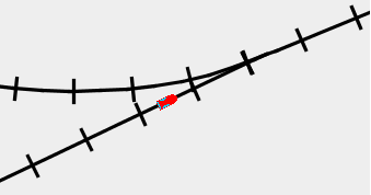
Select Line Color→Toggle visible slots to make guideway slots visible. Hermes uses synchronous clear path control where every vehicle is allowed to move only inside preallocated slots. By viewing these slots one can get a better understanding on how simulator works

A vehicle runs (almost) always in a slot

Select City Map→Black background to paint a black background instead of the city map (colored lines are viewed better against black background)

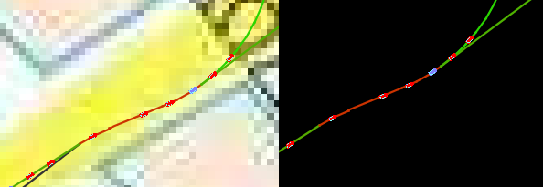
Map / Black background

Blue vehicles are empty . Red vehicles carry passengers

Options

Select Options→Set Options to set vehicle headway and speed.

Note that the < slot size >=< headway >X< speed > cannot be larger than 30 meters, because simulator uses synchronous clear path control which doesn't handle big slot sizes well.

Also note that if slot size is very small you may observe some visual artifacts during simulation like the figure below:

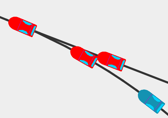
This doesn't mean that the vehicles collided. You may read the appendix for additional info on logical guideways

Actions

Select Action→Clear Statistics to clear all data gathered so far. You will need this if you want the network traffic to reach a stable state before you start collecting data.

Select Action→End Simulation in order to proceed to Presenter.

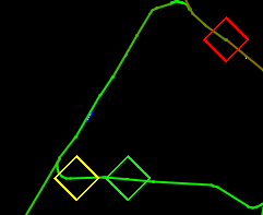
Select Action→Generate Follow Group in order to create a group at a specific station going to a specfic destination station . Source station will be marked with a green tilted square. Destination station will be marked with a red tilted square. The vehicle carrying the group will be marked with a yellow tilted square.

Select Action→Cancel Follow Group to stop following that group

Select Action→Vehicle malfunction and click on a vehicle on the main guideway in order to force that vehicle to stop. Normal service will stop , simulator will try to reroute existing vehicles without accepting any new ones. When all vehicles have stopped simulation will stop and a summary on the emergency event will be presented. (read the appendix for additional info on emergency mode)

Demand

Each Hermes vehicle can carry 1-2 persons . We call this small team a group.

There are 3 different ways to set the the flow of groups (demand) that will try to use the network during simulation.

1. Selecting areas of a city and adjust the number of trips that are generated or attracted to these areas
2. Setting the number of incoming and outgoing groups at each station
3. Setting the flow of groups between each pair of stations individually (demand matrix)

Selecting areas

The city area is divided into squares with size 100 meters X 100 meters, called cells. A cell that is near a station (less than 400 meters away) is an active cell. The area comprised of active cells (the part of the map which is less than 400 meters away from a station) is the network service area.  

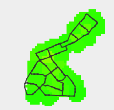
active cells (green)

Active cells generate groups . Each cell has a generating rate. A cell with generating rate e.g. 5 generates 5 groups/hour (that is an average value – actual generations are based on a pseudorandom function). These 5 groups will use the closest station as their origin station.

Active cells also attract groups. Each cell has an attraction rate. Cells with bigger rates will attract proportionably more groups. Groups attracted to a cell will use the closest to the cell station as their destination station.

Finally there is another factor that governs the demand: trip classes. Imagine you want to go to work: You ‘ll probably go there even if it is 30 km away. However if you want to buy cigarettes or bread for example , any local store will do fine , you won't go far away. This is why usually short trips are more often than long ones.

Trip classes are introduced in order to model the fact that some trips won’t go very far while others will. Each trip class has a range and an acceptance percentage. For example:

This is how this table is used:
A group is generated and must choose its destination. It randomly selects a cell (cells with bigger attraction rates have proportionably bigger chance of being selected). Distance is calculated and its trip class is defined. This trip has <accept> chance of being accepted . If not accepted the group tries again to find a destination.

Examples:

• A destination is selected which is 500 meters away. Chances are that people will rather walk such a small distance , therefore the corresponding class (class 1) has a <accept> = 30% . There is 30% chance this trip will materialize and 70% chance that the group will pick another destination.
• A destination is selected which is 2km away. The corresponding class (class 2) has a <accept> = 90% . The reasoning is that whatever the reason for the trip (work , buying something at a store) , the group won’t find a shorter way of doing it ,so it will rather accept it.
• A destination is selected which is 20km away. The corresponding class (class 3) has a <accept> = 40% . The reasoning is that the group will travel that distance only for a good reason (e.g. work ,visit a friend) rather than a trivial one (buying a chocolate bar).

Setting the demand

Select Demand→Generating Cells to edit the generating rate of cells. The cells on the map are colored according to their generating rate values (green=minValue , red=maxValue). Click on a point on the map and drag a circle (this way you select cells in an area) . A popup window will emerge showing information about the selected cells. It also shows: “Selected area (x,y),r” where x,y are the coordinates of the circle center , r is its radius. Type a value (positive or negative) in the edit box . This value will be EQUALLY DISTRIBUTED among all selected cells. Press “ESC” to exit generating cells mode.

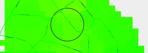
Drawing a circle to select cells

Select Demand→Attraction Cells to edit the attraction rate of cells. Cells are colored according to their attraction values. Click and drag a circle to select cells. Type a value (positive or negative) that will be ADDED TO EACH cell. Press “ESC” to exit attraction cells mode.

Select Demand→Trip Classes to edit the trip classes.

Select Demand→Show Station Rates to see an estimation of group traffic for each station.

You ‘ll get a report comprising of lines like this:

Station 166 : (7200,3000)   Generates : 100 groups/hour    Receives : 89 groups/hour   Group attraction : 9990 Source:5 Sink:7

Which tells you that station 166 , at coordinates 7200,3000 , generates about 100 groups per hour and receives about 89 groups per hour. Its relative attraction (compared to other stations) is 9990. (groups generated and attracted by the cells that this station services). Capacitor number 5 provides empty vehicles for this station. Capacitor number 7 handles any surplus vehicles from this station.

Default values

Generation rate: an initial generating rate of 100*<number of stations> groups/hour is divided equally among cells.
Attraction rate: attraction rate of all cells is set to 100.

Using a Demand Program:

You can edit the demand as you go on with the simulation. However if you want to simulate the same scenario many times, making adjustments, you should better create a demand program and load it each time you perform a simulation.

A demand program is a .txt file containing statements:

Available statements are:

Example of a demand program:

areas
// set the trip classes (optional)
class 1000 30
class 10000 90
class 15000 40
// produce extra 100000 groups/hour on the city at time 1
generate 3 10000 10000 20000 100000
// add 1000 attraction to each cell in the CBD at time 2
attract 4 10000 10000 2000 1000
// wait until the network comes to a stable state
// then clear statistics
clear 1000
// gather some data from the stable phase,then pause
pause 2000

A demand program can contain any number of statements , even only 1. The demand program's first line must denote its type: In this case the keyword 'areas'.

Select Demand→Demand Program to load a demand program. Note that you cannot load a demand program once the simulation has started.

Setting flow of groups at each station

Available statements are:

Example of a demand program:

rates
// set the trip classes (optional)
class 1000 30
class 10000 90
class 15000 40
// set station generating group rates explicitly: station1=100 station2=150 station3=200
setStationGeneration 1 100 150 200
// set station attraction rates explicitly: station1=10000 station2=15000 station3=20000
setStationAttraction 2 10000 15000 20000
// wait until the network comes to a stable state
// then clear statistics
clear 1000
// gather some data from the stable phase,then pause
pause 2000

Note that the demand program's first line must denote its type: In this case the keyword 'rates'.

Default values

Generation rate: initial generating rate for each station is set to 100 groups/hour
Attraction rate: attraction rate for each station is set to 100.

Setting the flow of each pair of stations individually (demand matrix)

Available statements are:

Example of a demand program:

odmatrix
//set group flow from station 1: to station1=0, to station2=10, to station3=20, to station4=30
setod 1 0 10 20 30
setod 2 15 0 25 35
setod 3 18 28 0 38
setod 4 6 16 36 0
// wait until the network comes to a stable state
// then clear statistics
clear 1000
// gather some data from the stable phase,then pause
pause 2000

Default values

Each flow between each pair of stations is set to 10 groups/hour

BACK